Detecting Blindness with Deep Learning
Using CNNs to detect diabetic retinopathy in retina photos

Last update: 09.06.2022. All opinions are my own.
1. Overview
Can deep learning help to detect blindness?
This blog post describes a project that develops a convolutional neural network (CNN) for predicting the severity of the diabetic retinopathy based on the patient's retina photos. The project was completed within the scope of the Udacity ML Engineer nano-degree program and the Kaggle competition hosted by the Asia Pacific Tele-Ophthalmology Society (APTOS). ^ The blog post provides a project walkthrough covering the following steps:
- data exploration and image preprocessing to normalize images from different clinics
- using transfer learning to pre-train CNN on a larger data set
- employing techniques such as learning rate scheduler, test-time augmentation and others
The modeling is performed in PyTorch. All notebooks and a PDF report are available on Github.
2. Motivation
Diabetic retinopathy (DR) is one of the leading causes of vision loss. The World Health Organization reports that more than 300 million people worldwide have diabetes (Wong et al. 2016). In 2019, the global prevalence of DR among individuals with diabetes was at more than 25% (Thomas et al. 2019). The prevalence has been rising rapidly in developing countries.
Early detection and treatment are crucial steps towards preventing DR. The screening procedure requires a trained clinical expert to examine the fundus photographs of the patient's retina. This creates delays in diagnosis and treatment. This is especially relevant for developing countries, which often lack qualified medical staff to perform the diagnosis. Automated detection of DR can speed up the efficiency and coverage of the screening programs.
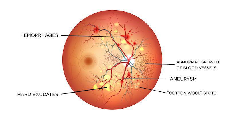
Image source: https://www.eyeops.com/contents/our-services/eye-diseases/diabetic-retinopathy
3. Data preparation
Data preparation is a very important step that is frequently underestimated. The quality of the input data has a strong impact on the resulting performance of the developed machine learning models. Therefore, it is crucial to take some time to look at the data and think about possible issues that should be addressed before moving on to the modeling stage. Let's do that!
Data exploration
The data set is available for the download at the competition's website. The data includes 3,662 labeled retina images of clinical patients and a test set with 1,928 images with unknown labels.
The images are labeled by a clinical expert. The integer labels indicate the severity of DR on a scale from 0 to 4, where 0 indicates no disease and 5 is the proliferative stage of DR.
Let's start by importing the data and looking at the class distribution.
#collapse-hide

##### PACKAGES

import numpy as np
import pandas as pd

import torch
import torchvision

from torchvision import transforms, datasets
from torch.utils.data import Dataset

from PIL import Image, ImageFile
ImageFile.LOAD_TRUNCATED_IMAGES = True
import cv2

from tqdm import tqdm_notebook as tqdm

import random
import time
import sys
import os
import math

import matplotlib.pyplot as plt
import seaborn as sns

pd.set_option('display.max_columns', None)
%matplotlib inline
import warnings
warnings.filterwarnings('ignore')


##### CLASS DISTRIBUTION

# import data
train = pd.read_csv('../input/aptos2019-blindness-detection/train.csv')
test  = pd.read_csv('../input/aptos2019-blindness-detection/sample_submission.csv')

# plot
fig = plt.figure(figsize = (15, 5))
plt.hist(train['diagnosis'])
plt.title('Class Distribution')
plt.ylabel('Number of examples')
plt.xlabel('Diagnosis')
The data is imbalanced: 49% images are from healthy patients. The remaining 51% are different stages of DR. The least common class is 3 (severe stage) with only 5% of the total examples.
The data is collected from multiple clinics using a variety of camera models, which creates discrepancies in the image resolution, aspect ratio and other parameters. This is demonstrated in the snippet below, where we plot histograms of image width, height and aspect ratio.
#collapse-hide

# placeholder
image_stats = []

# import loop
for index, observation in tqdm(train.iterrows(), total = len(train)):

    # import image
    img = cv2.imread('../input/aptos2019-blindness-detection/train_images/{}.png'.format(observation['id_code']))

    # compute stats
    height, width, channels = img.shape
    ratio = width / height

    # save
    image_stats.append(np.array((observation['diagnosis'], height, width, channels, ratio)))

# construct DF
image_stats = pd.DataFrame(image_stats)
image_stats.columns = ['diagnosis', 'height', 'width', 'channels', 'ratio']

# create plot
fig = plt.figure(figsize = (15, 5))

# width
plt.subplot(1, 3, 1)
plt.hist(image_stats['width'])
plt.title('(a) Image Width')
plt.ylabel('Number of examples')
plt.xlabel('Width')

# height
plt.subplot(1, 3, 2)
plt.hist(image_stats['height'])
plt.title('(b) Image Height')
plt.ylabel('Number of examples')
plt.xlabel('Height')

# ratio
plt.subplot(1, 3, 3)
plt.hist(image_stats['ratio'])
plt.title('(c) Aspect Ratio')
plt.ylabel('Number of examples')
plt.xlabel('Ratio')
Now, let's look into the actual eyes! The code below creates the EyeData dataset class to import images. We also create a DataLoader object to load sample images and visualize the first batch.
#collapse-hide

##### DATASET

# image preprocessing
def prepare_image(path, image_size = 256):

    # import
    image = cv2.imread(path)
    image = cv2.cvtColor(image, cv2.COLOR_BGR2RGB)

    # resize
    image = cv2.resize(image, (int(image_size), int(image_size)))

    # convert to tensor
    image = torch.tensor(image)
    image = image.permute(2, 1, 0)
    return image

# dataset
class EyeData(Dataset):

    # initialize
    def __init__(self, data, directory, transform = None):
        self.data      = data
        self.directory = directory
        self.transform = transform

    # length
    def __len__(self):
        return len(self.data)

    # get items
    def __getitem__(self, idx):
        img_name = os.path.join(self.directory, self.data.loc[idx, 'id_code'] + '.png')
        image    = prepare_image(img_name)
        image    = self.transform(image)
        label    = torch.tensor(self.data.loc[idx, 'diagnosis'])
        return {'image': image, 'label': label}


##### EXAMINE SAMPLE BATCH

# transformations
sample_trans = transforms.Compose([transforms.ToPILImage(),
                                   transforms.ToTensor(),
                                  ])

# dataset
sample = EyeData(data       = train,
                 directory  = '../input/aptos2019-blindness-detection/train_images',
                 transform  = sample_trans)

# data loader
sample_loader = torch.utils.data.DataLoader(dataset     = sample,
                                            batch_size  = 10,
                                            shuffle     = False,
                                            num_workers = 4)

# display images
for batch_i, data in enumerate(sample_loader):

    # extract data
    inputs = data['image']
    labels = data['label'].view(-1, 1)

    # create plot
    fig = plt.figure(figsize = (15, 7))
    for i in range(len(labels)):
        ax = fig.add_subplot(2, len(labels)/2, i + 1, xticks = [], yticks = [])
        plt.imshow(inputs[i].numpy().transpose(1, 2, 0))
        ax.set_title(labels.numpy()[i])

    break
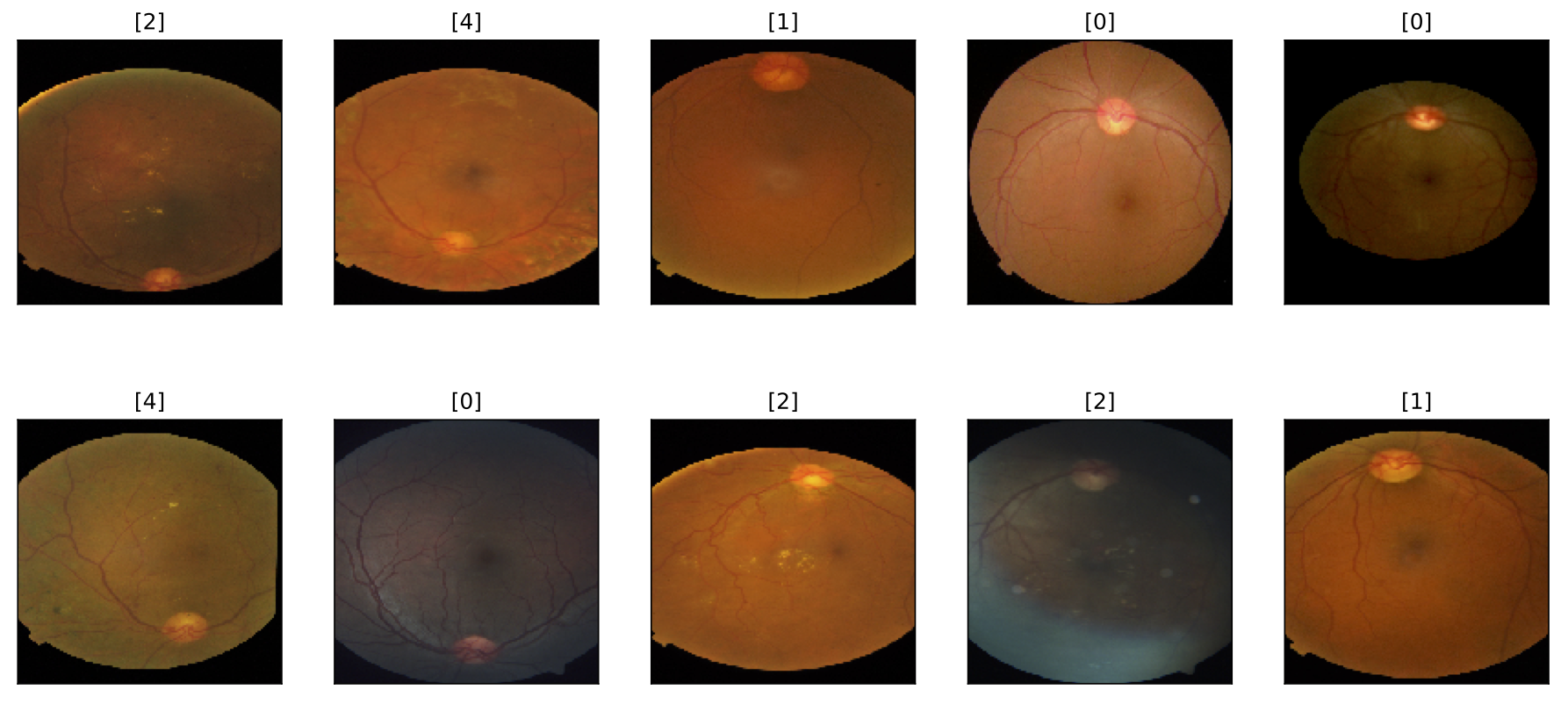
The illustration further emphasizes differences in the aspect ratio and lighting conditions.
The severity of DR is diagnosed by the presence of visual cues such as abnormal blood vessels, hard exudates and so-called cotton wool spots. You can read more about the diagnosing process here. Comparing the sample images, we can see the presence of exudates and cotton wool spots on some of the retina images of sick patients.
Image preprocessing
To simplify the classification task for our model, we need to ensure that retina images look similar.
First, using cameras with different aspect ratios results in some images having large black areas around the eye. The black areas do not contain information relevant for prediction and can be cropped. However, the size of black areas varies from one image to another. To address this, we develop a cropping function that converts the image to grayscale and marks black areas based on the pixel intensity. Next, we find a mask of the image by selecting rows and columns in which all pixels exceed the intensity threshold. This helps to remove vertical or horizontal rectangles filled with black similar to the ones observed in the upper-right image. After removing the black stripes, we resize the images to the same height and width.
Another issue is the eye shape. Depending on the image parameters, some eyes have a circular form, whereas others look like ovals. Since the size and shape of cues located in the retina determine the disease severity, it is crucial to standardize the eye shape as well. To do so, we develop another function that makes a circular crop around the center of the image.
Finally, we correct for the lightning and brightness discrepancies by smoothing the images using a Gaussian filter.
The snippet below provides the updated prepare_image() function that incorporates the discussed preprocessing steps.
#collapse-show

### image preprocessing function
def prepare_image(path, sigmaX = 10, do_random_crop = False):

    # import image
    image = cv2.imread(path)
    image = cv2.cvtColor(image, cv2.COLOR_BGR2RGB)

    # perform smart crops
    image = crop_black(image, tol = 7)
    if do_random_crop == True:
        image = random_crop(image, size = (0.9, 1))

    # resize and color
    image = cv2.resize(image, (int(image_size), int(image_size)))
    image = cv2.addWeighted(image, 4, cv2.GaussianBlur(image, (0, 0), sigmaX), -4, 128)

    # circular crop
    image = circle_crop(image, sigmaX = sigmaX)

    # convert to tensor
    image = torch.tensor(image)
    image = image.permute(2, 1, 0)
    return image


### automatic crop of black areas
def crop_black(img, tol = 7):

    if img.ndim == 2:
        mask = img > tol
        return img[np.ix_(mask.any(1),mask.any(0))]

    elif img.ndim == 3:
        gray_img = cv2.cvtColor(img, cv2.COLOR_RGB2GRAY)
        mask = gray_img > tol
        check_shape = img[:,:,0][np.ix_(mask.any(1),mask.any(0))].shape[0]

        if (check_shape == 0):
            return img
        else:
            img1 = img[:,:,0][np.ix_(mask.any(1),mask.any(0))]
            img2 = img[:,:,1][np.ix_(mask.any(1),mask.any(0))]
            img3 = img[:,:,2][np.ix_(mask.any(1),mask.any(0))]
            img  = np.stack([img1, img2, img3], axis = -1)
            return img


### circular crop around center
def circle_crop(img, sigmaX = 10):

    height, width, depth = img.shape

    largest_side = np.max((height, width))
    img = cv2.resize(img, (largest_side, largest_side))

    height, width, depth = img.shape

    x = int(width / 2)
    y = int(height / 2)
    r = np.amin((x,y))

    circle_img = np.zeros((height, width), np.uint8)
    cv2.circle(circle_img, (x,y), int(r), 1, thickness = -1)

    img = cv2.bitwise_and(img, img, mask = circle_img)
    return img


### random crop
def random_crop(img, size = (0.9, 1)):

    height, width, depth = img.shape

    cut = 1 - random.uniform(size[0], size[1])

    i = random.randint(0, int(cut * height))
    j = random.randint(0, int(cut * width))
    h = i + int((1 - cut) * height)
    w = j + int((1 - cut) * width)

    img = img[i:h, j:w, :]

    return img
Next, we define a new EyeData class that uses the new processing functions and visualize a batch of sample images after corrections.
#collapse-show

##### DATASET

# dataset class
class EyeData(Dataset):

    # initialize
    def __init__(self, data, directory, transform = None):
        self.data      = data
        self.directory = directory
        self.transform = transform

    # length
    def __len__(self):
        return len(self.data)

    # get items
    def __getitem__(self, idx):
        img_name = os.path.join(self.directory, self.data.loc[idx, 'id_code'] + '.png')
        image    = prepare_image(img_name)
        image    = self.transform(image)
        label    = torch.tensor(self.data.loc[idx, 'diagnosis'])
        return {'image': image, 'label': label}


##### EXAMINE SAMPLE BATCH

image_size = 256


# transformations
sample_trans = transforms.Compose([transforms.ToPILImage(),
                                   transforms.ToTensor(),
                                  ])

# dataset
sample = EyeData(data       = train,
                 directory  = '../input/aptos2019-blindness-detection/train_images',
                 transform  = sample_trans)

# data loader
sample_loader = torch.utils.data.DataLoader(dataset     = sample,
                                            batch_size  = 10,
                                            shuffle     = False,
                                            num_workers = 4)

# display images
for batch_i, data in enumerate(sample_loader):

    # extract data
    inputs = data['image']
    labels = data['label'].view(-1, 1)

    # create plot
    fig = plt.figure(figsize = (15, 7))
    for i in range(len(labels)):
        ax = fig.add_subplot(2, len(labels)/2, i + 1, xticks = [], yticks = [])
        plt.imshow(inputs[i].numpy().transpose(1, 2, 0))
        ax.set_title(labels.numpy()[i])

    break
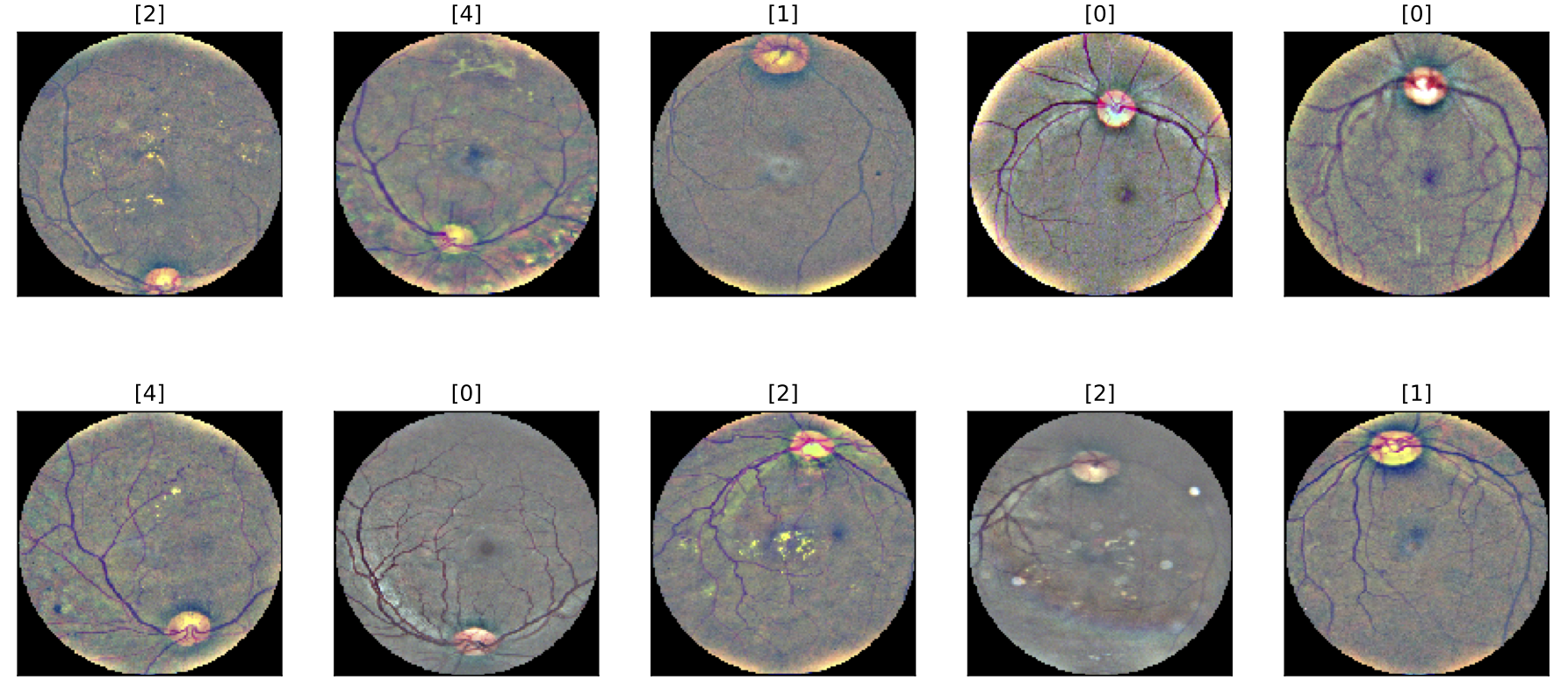
This looks much better! Comparing the retina images to the ones before the preprocessing, we can see that the apparent discrepancies between the photos are now fixed. The eyes now have a similar circular shape, and the color scheme is more consistent. This should help the model to detect the signs of the DR.
Check out this notebook by Nakhon Ratchasima for more ideas on the image preprocessing for retina photos. The functions in this project are largely inspired by his work during the competition.
4. Modeling
CNNs achieve state-of-the-art performance in computer vision tasks. Recent medical research also shows a high potential of CNNs in DR classification (Gulshan et al. 2016).
In this project, we employ a CNN model with the EfficientNet architecture. EfficientNet is one of the recent state-of-the-art image classification models (Tan et al. 2019). It encompasses 8 architecture variants (B0 to B7) that differ in the model complexity and default image size.
The architecture of EfficientNet B0 is visualized below. We test multiple EfficientNet architectures and use the one that demonstrates the best performance.

The modeling pipeline consists of three stages:
- Pre-training. The data set has a limited number of images (N = 3,662). We pre-train the CNN model on a larger data set from the previous Kaggle competition.
- Fine-tuning. We fine-tune the model on the target data set. We use cross-validation and make modeling decisions based on the performance of the out-of-fold predictions.
- Inference. We aggregate predictions of the models trained on different combinations of training folds and use test-time augmentation to further improve the performance.
Pre-training
Due to small sample size, we can not train a complex neural architecture from scratch. This is where transfer learning comes in handy. The idea of transfer learning is to pre-train a model on a different data (source domain) and fine-tune it on a relevant data set (target domain).
A good candidate for the source domain is the ImageNet database. Most published CNN models are trained on that data. However, ImageNet images are substantially different from the retina images we want to classify. Although initializing CNN with ImageNet weights might help the network to transfer the knowledge of basic image patterns such as shapes and edges, we still need to learn a lot from the target domain.
It turns out that APTOS had hosted another Kaggle competition on the DR classification in 2015. The data set of the 2015 competition features 35,126 retina images labeled by a clinician using the same scale as the target data set. The data is available for the download here.
This enables us to use following pipeline:
- initialize weights from a CNN trained on ImageNet
- train the CNN on the 2015 data set
- fine-tune the CNN on the 2019 data set
Let's start modeling! First, we enable GPU support and fix random seeds. The function seed_everything() sets seed for multiple packages, including numpy and pytorch, to ensure reproducibility.
#collapse-show

# GPU check
train_on_gpu = torch.cuda.is_available()
if not train_on_gpu:
    print('CUDA is not available. Training on CPU...')
    device = torch.device('cpu')
else:
    print('CUDA is available. Training on GPU...')
    device = torch.device('cuda:0')

# set seed
def seed_everything(seed = 23):
    os.environ['PYTHONHASHSEED'] = str(seed)
    random.seed(seed)
    np.random.seed(seed)
    torch.manual_seed(seed)
    torch.cuda.manual_seed(seed)
    torch.backends.cudnn.deterministic = True
    torch.backends.cudnn.benchmark = False
seed = 23
seed_everything(seed)
Let's take a quick look at the class distribution in the 2015 data.
#collapse-show

# import data
train = pd.read_csv('../input/diabetic-retinopathy-resized/trainLabels.csv')
train.columns = ['id_code', 'diagnosis']
test = pd.read_csv('../input/aptos2019-blindness-detection/train.csv')

# check shape
print(train.shape, test.shape)
print('-' * 15)
print(train['diagnosis'].value_counts(normalize = True))
print('-' * 15)
print(test['diagnosis'].value_counts(normalize = True))
The imbalance in the source data is stronger than in the target data: 73% of images represent healthy patients, whereas the most severe stage of the DR is only found in 2% of the images. To address the imbalance, we will use the target data set as a validation sample during training.
We create two Dataset objects to enable different augmentations on training and inference stages: EyeTrainData and EyeTestData. The former includes a random crop that is skipped for the test data.
#collapse-hide

# dataset class: train
class EyeTrainData(Dataset):

    # initialize
    def __init__(self, data, directory, transform = None):
        self.data      = data
        self.directory = directory
        self.transform = transform

    # length
    def __len__(self):
        return len(self.data)

    # get items
    def __getitem__(self, idx):
        img_name = os.path.join(self.directory, self.data.loc[idx, 'id_code'] + '.jpeg')
        image    = prepare_image(img_name, do_random_crop = True)
        image    = self.transform(image)
        label    = torch.tensor(self.data.loc[idx, 'diagnosis'])
        return {'image': image, 'label': label}


# dataset class: test
class EyeTestData(Dataset):

    # initialize
    def __init__(self, data, directory, transform = None):
        self.data      = data
        self.directory = directory
        self.transform = transform

    # length
    def __len__(self):
        return len(self.data)

    # get items
    def __getitem__(self, idx):
        img_name = os.path.join(self.directory, self.data.loc[idx, 'id_code'] + '.png')
        image    = prepare_image(img_name, do_random_crop = False)
        image    = self.transform(image)
        label    = torch.tensor(self.data.loc[idx, 'diagnosis'])
        return {'image': image, 'label': label}
We use a batch size of 20 and set the image size of 256. The choice of these parameters is a trade-off between performance and resource capacity. Feel free to try larger image and batch sizes if you have resources.
We use the following data augmentations during training:
- random horizontal flip
- random vertical flip
- random rotation in the range [-360 degrees, 360 degrees]
#collapse-show

# parameters
batch_size = 20
image_size = 256

# train transformations
train_trans = transforms.Compose([transforms.ToPILImage(),
                                  transforms.RandomRotation((-360, 360)),
                                  transforms.RandomHorizontalFlip(),
                                  transforms.RandomVerticalFlip(),
                                  transforms.ToTensor()
                                 ])

# validation transformations
valid_trans = transforms.Compose([transforms.ToPILImage(),
                                  transforms.ToTensor(),
                                 ])

# create datasets
train_dataset = EyeTrainData(data      = train,
                             directory = '../input/diabetic-retinopathy-resized/resized_train/resized_train',
                             transform = train_trans)
valid_dataset = EyeTestData(data       = test,
                            directory  = '../input/aptos2019-blindness-detection/train_images',
                            transform  = valid_trans)

# create data loaders
train_loader = torch.utils.data.DataLoader(train_dataset,
                                           batch_size  = batch_size,
                                           shuffle     = True,
                                           num_workers = 4)
valid_loader = torch.utils.data.DataLoader(valid_dataset,
                                           batch_size  = batch_size,
                                           shuffle     = False,
                                           num_workers = 4)
Next, let's instantiate the EfficentNet model. We use B4 architecture and initialize pre-trained ImageNet weights by downloading the model parameters in the PyTorch format. The convolutional part of the network responsible for feature extraction outputs a tensor with 1792 features. To adapt the CNN to our task, we replace the last fully-connected classification layer with a (1792, 5) fully-connected layer.
The CNN is instantiated with init_model(). The argument train ensures that we load ImageNet weights on the training stage and turn off gradient computation on the inference stage.
#collapse-show

# model name
model_name = 'enet_b4'

# initialization function
def init_model(train = True):

    ### training mode
    if train == True:

        # load pre-trained model
        model = EfficientNet.from_pretrained('efficientnet-b4', num_classes = 5)


    ### inference mode
    if train == False:

        # load pre-trained model
        model = EfficientNet.from_name('efficientnet-b4')
        model._fc = nn.Linear(model._fc.in_features, 5)

        # freeze  layers
        for param in model.parameters():
            param.requires_grad = False

    return model


# check architecture
model = init_model()
print(model)
Since we are dealing with a multiple classification problem, we use cross-entropy as a loss function. We use nn.CrossEntropyLoss() which combines logsoftmax and negative log-likelihood loss and applies them to the output of the last network layer.
The Kaggle competition uses Cohen's kappa for evaluation. Kappa measures the agreement between the actual and predicted labels. Since Kappa is non-differentiable, we can not use it as a loss function. At the same time, we can use Kappa to evaluate the performance and early stop the training epochs.
We use Adam optimizer with a starting learning rate of 0.001. During training, we use a learning rate scheduler, which multiplies the learning rate by 0.5 after every 5 epochs. This helps to make smaller changes to the network weights when we are getting closer to the optimum.
#collapse-show

# loss function
criterion = nn.CrossEntropyLoss()

# epochs
max_epochs = 15
early_stop = 5

# learning rates
eta = 1e-3

# scheduler
step  = 5
gamma = 0.5

# optimizer
optimizer = optim.Adam(model.parameters(), lr = eta)
scheduler = lr_scheduler.StepLR(optimizer, step_size = step, gamma = gamma)

# initialize model and send to GPU
model = init_model()
model = model.to(device)
After each training epoch, we validate the model on the target data. We extract class scores from the last fully-connected layer and predict the image class corresponding to the highest score. We train the network for 15 epochs, tracking the validation loss and Cohen's kappa. If the kappa does not increase for 5 consecutive epochs, we terminate the training process and save model weights for the epoch associated with the highest validation kappa.
#collapse-show

# placeholders
oof_preds = np.zeros((len(test), 5))
val_kappas = []
val_losses = []
trn_losses = []
bad_epochs = 0

# timer
cv_start = time.time()

# training and validation loop
for epoch in range(max_epochs):

    ##### PREPARATION

    # timer
    epoch_start = time.time()

    # reset losses
    trn_loss = 0.0
    val_loss = 0.0

    # placeholders
    fold_preds = np.zeros((len(test), 5))


    ##### TRAINING

    # switch regime
    model.train()

    # loop through batches
    for batch_i, data in enumerate(train_loader):

        # extract inputs and labels
        inputs = data['image']
        labels = data['label'].view(-1)
        inputs = inputs.to(device, dtype = torch.float)
        labels = labels.to(device, dtype = torch.long)
        optimizer.zero_grad()

        # forward and backward pass
        with torch.set_grad_enabled(True):
            preds = model(inputs)
            loss  = criterion(preds, labels)
            loss.backward()
            optimizer.step()

        # compute loss
        trn_loss += loss.item() * inputs.size(0)


    ##### INFERENCE

    # switch regime
    model.eval()

    # loop through batches
    for batch_i, data in enumerate(valid_loader):

        # extract inputs and labels
        inputs = data['image']
        labels = data['label'].view(-1)
        inputs = inputs.to(device, dtype = torch.float)
        labels = labels.to(device, dtype = torch.long)

        # compute predictions
        with torch.set_grad_enabled(False):
            preds = model(inputs).detach()
            fold_preds[batch_i * batch_size:(batch_i + 1) * batch_size, :] = preds.cpu().numpy()

        # compute loss
        loss      = criterion(preds, labels)
        val_loss += loss.item() * inputs.size(0)

    # save predictions
    oof_preds = fold_preds

    # scheduler step
    scheduler.step()


    ##### EVALUATION

    # evaluate performance
    fold_preds_round = fold_preds.argmax(axis = 1)
    val_kappa = metrics.cohen_kappa_score(test['diagnosis'], fold_preds_round.astype('int'), weights = 'quadratic')

    # save perfoirmance values
    val_kappas.append(val_kappa)
    val_losses.append(val_loss / len(test))
    trn_losses.append(trn_loss / len(train))


    ##### EARLY STOPPING

    # display info
    print('- epoch {}/{} | lr = {} | trn_loss = {:.4f} | val_loss = {:.4f} | val_kappa = {:.4f} | {:.2f} min'.format(
        epoch + 1, max_epochs, scheduler.get_lr()[len(scheduler.get_lr()) - 1],
        trn_loss / len(train), val_loss / len(test), val_kappa,
        (time.time() - epoch_start) / 60))

    # check if there is any improvement
    if epoch > 0:
        if val_kappas[epoch] < val_kappas[epoch - bad_epochs - 1]:
            bad_epochs += 1
        else:
            bad_epochs = 0

    # save model weights if improvement
    if bad_epochs == 0:
        oof_preds_best = oof_preds.copy()
        torch.save(model.state_dict(), '../models/model_{}.bin'.format(model_name))

    # break if early stop
    if bad_epochs == early_stop:
        print('Early stopping. Best results: loss = {:.4f}, kappa = {:.4f} (epoch {})'.format(
            np.min(val_losses), val_kappas[np.argmin(val_losses)], np.argmin(val_losses) + 1))
        print('')
        break

    # break if max epochs
    if epoch == (max_epochs - 1):
        print('Did not met early stopping. Best results: loss = {:.4f}, kappa = {:.4f} (epoch {})'.format(
            np.min(val_losses), val_kappas[np.argmin(val_losses)], np.argmin(val_losses) + 1))
        print('')
        break

# load best predictions
oof_preds = oof_preds_best

# print performance
print('')
print('Finished in {:.2f} minutes'.format((time.time() - cv_start) / 60))
Training on the Kaggle GPU-enabled machine took us about 7 hours! Let's visualize the training and validation loss dynamics.
#collapse-show

# plot size
fig = plt.figure(figsize = (15, 5))

# plot loss dynamics
plt.subplot(1, 2, 1)
plt.plot(trn_losses, 'red',   label = 'Training')
plt.plot(val_losses, 'green', label = 'Validation')
plt.xlabel('Epoch')
plt.ylabel('Loss')
plt.legend()

# plot kappa dynamics
plt.subplot(1, 2, 2)
plt.plot(val_kappas, 'blue', label = 'Kappa')
plt.xlabel('Epoch')
plt.ylabel('Kappa')
plt.legend()
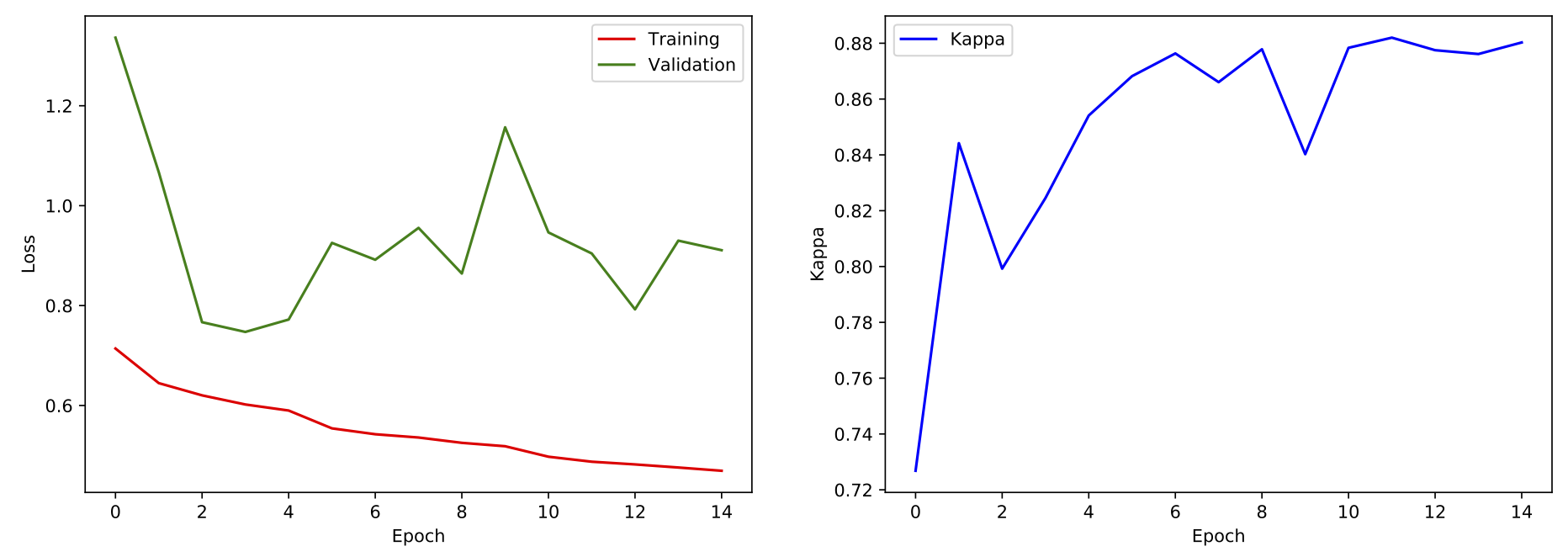
The cross-entropy loss on the validation set reaches minimum already after 3 epochs. At the same time, kappa continues to increase up to the 15th epoch. Since we use kappa to evaluate the quality of our solution, we save weights after 15 epochs.
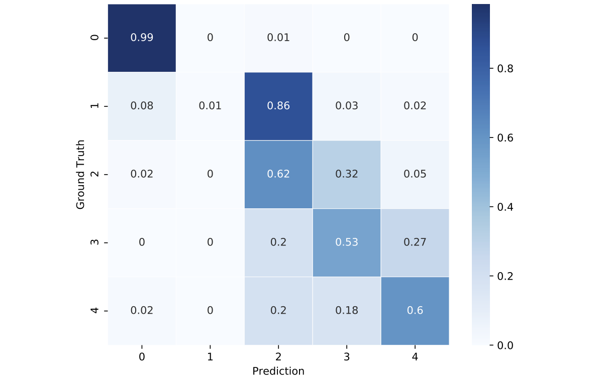
We also construct a confusion matrix of the trained model. The numbers in the cells are percentages. According to the results, the model does a poor job in distinguishing the mild and moderate stages of DR: 86% of images with mild DR are classified as moderate. The best performance is observed for healthy patients. Overall, we see that the model tends to confuse nearby severity stages but rarely misclassifies the proliferate and mild stages.
Fine-tuning on the target data is performed within 4-fold cross-validation. To ensure that we have enough examples of each class, we perform cross-validation with stratification.
On each iteration, we instantiate the EfficientNet B4 model with the same architecture as in the previous section. Next, we load the saved weights from the model pre-trained on the source data. We freeze weights on all network layers except for the last fully-connected layer. The weights in this layer are fine-tuned. As on the pre-training stage, we use Adam optimizer and implement a learning rate scheduler. We also track performance on the validation folds and stop training if kappa does not increase for 5 consecutive epochs.
The process is repeated for each of the 4 folds, and the best model weights are saved for each combination of the training folds.
The init_model() is updated to load the weights saved on the pre-training stage and freeze the first layers of the network in the training regime.
#collapse-show

# model name
model_name = 'enet_b4'

# initialization function
def init_model(train = True, trn_layers = 2):

    ### training mode
    if train == True:

        # load pre-trained model
        model = EfficientNet.from_pretrained('efficientnet-b4', num_classes = 5)
        model.load_state_dict(torch.load('../models/model_{}.bin'.format(model_name, 1)))

        # freeze first layers
        for child in list(model.children())[:-trn_layers]:
            for param in child.parameters():
                param.requires_grad = False


    ### inference mode
    if train == False:

        # load pre-trained model
        model = EfficientNet.from_pretrained('efficientnet-b4', num_classes = 5)
        model.load_state_dict(torch.load('../models/model_{}.bin'.format(model_name, 1)))

        # freeze all layers
        for param in model.parameters():
            param.requires_grad = False

    return model


# check architecture
model = init_model()
The training loop is now wrapped into a cross-validation loop.
#collapse-hide

##### VALIDATION SETTINGS

# no. folds
num_folds = 4

# creating splits
skf    = StratifiedKFold(n_splits = num_folds, shuffle = True, random_state = seed)
splits = list(skf.split(train['id_code'], train['diagnosis']))

# placeholders
oof_preds = np.zeros((len(train), 1))

# timer
cv_start = time.time()


##### PARAMETERS

# loss function
criterion = nn.CrossEntropyLoss()

# epochs
max_epochs = 15
early_stop = 5

# learning rates
eta = 1e-3

# scheduler
step  = 5
gamma = 0.5


##### CROSS-VALIDATION LOOP
for fold in tqdm(range(num_folds)):

    ####### DATA PREPARATION

    # display information
    print('-' * 30)
    print('FOLD {}/{}'.format(fold + 1, num_folds))
    print('-' * 30)

    # load splits
    data_train = train.iloc[splits[fold][0]].reset_index(drop = True)
    data_valid = train.iloc[splits[fold][1]].reset_index(drop = True)

    # create datasets
    train_dataset = EyeTrainData(data      = data_train,
                                 directory = '../input/aptos2019-blindness-detection/train_images',
                                 transform = train_trans)
    valid_dataset = EyeTrainData(data      = data_valid,
                                 directory = '../input/aptos2019-blindness-detection/train_images',
                                 transform = valid_trans)

    # create data loaders
    train_loader = torch.utils.data.DataLoader(train_dataset,
                                               batch_size  = batch_size,
                                               shuffle     = True,
                                               num_workers = 4)
    valid_loader = torch.utils.data.DataLoader(valid_dataset,
                                               batch_size  = batch_size,
                                               shuffle     = False,
                                               num_workers = 4)


    ####### MODEL PREPARATION

    # placeholders
    val_kappas = []
    val_losses = []
    trn_losses = []
    bad_epochs = 0

    # load best OOF predictions
    if fold > 0:
        oof_preds = oof_preds_best.copy()

    # initialize and send to GPU
    model = init_model(train = True)
    model = model.to(device)

    # optimizer
    optimizer = optim.Adam(model._fc.parameters(), lr = eta)
    scheduler = lr_scheduler.StepLR(optimizer, step_size = step, gamma = gamma)


    ####### TRAINING AND VALIDATION LOOP
    for epoch in range(max_epochs):

        ##### PREPARATION

        # timer
        epoch_start = time.time()

        # reset losses
        trn_loss = 0.0
        val_loss = 0.0

        # placeholders
        fold_preds = np.zeros((len(data_valid), 1))


        ##### TRAINING

        # switch regime
        model.train()

        # loop through batches
        for batch_i, data in enumerate(train_loader):

            # extract inputs and labels
            inputs = data['image']
            labels = data['label'].view(-1)
            inputs = inputs.to(device, dtype = torch.float)
            labels = labels.to(device, dtype = torch.long)
            optimizer.zero_grad()

            # forward and backward pass
            with torch.set_grad_enabled(True):
                preds = model(inputs)
                loss  = criterion(preds, labels)
                loss.backward()
                optimizer.step()

            # compute loss
            trn_loss += loss.item() * inputs.size(0)


        ##### INFERENCE

        # initialize
        model.eval()

        # loop through batches
        for batch_i, data in enumerate(valid_loader):

            # extract inputs and labels
            inputs = data['image']
            labels = data['label'].view(-1)
            inputs = inputs.to(device, dtype = torch.float)
            labels = labels.to(device, dtype = torch.long)

            # compute predictions
            with torch.set_grad_enabled(False):
                preds = model(inputs).detach()
                _, class_preds = preds.topk(1)
                fold_preds[batch_i * batch_size:(batch_i + 1) * batch_size, :] = class_preds.cpu().numpy()

            # compute loss
            loss      = criterion(preds, labels)
            val_loss += loss.item() * inputs.size(0)

        # save predictions
        oof_preds[splits[fold][1]] = fold_preds

        # scheduler step
        scheduler.step()


        ##### EVALUATION

        # evaluate performance
        fold_preds_round = fold_preds
        val_kappa = metrics.cohen_kappa_score(data_valid['diagnosis'], fold_preds_round.astype('int'), weights = 'quadratic')

        # save perfoirmance values
        val_kappas.append(val_kappa)
        val_losses.append(val_loss / len(data_valid))
        trn_losses.append(trn_loss / len(data_train))


        ##### EARLY STOPPING

        # display info
        print('- epoch {}/{} | lr = {} | trn_loss = {:.4f} | val_loss = {:.4f} | val_kappa = {:.4f} | {:.2f} min'.format(
            epoch + 1, max_epochs, scheduler.get_lr()[len(scheduler.get_lr()) - 1],
            trn_loss / len(data_train), val_loss / len(data_valid), val_kappa,
            (time.time() - epoch_start) / 60))

        # check if there is any improvement
        if epoch > 0:
            if val_kappas[epoch] < val_kappas[epoch - bad_epochs - 1]:
                bad_epochs += 1
            else:
                bad_epochs = 0

        # save model weights if improvement
        if bad_epochs == 0:
            oof_preds_best = oof_preds.copy()
            torch.save(model.state_dict(), '../models/model_{}_fold{}.bin'.format(model_name, fold + 1))

        # break if early stop
        if bad_epochs == early_stop:
            print('Early stopping. Best results: loss = {:.4f}, kappa = {:.4f} (epoch {})'.format(
                np.min(val_losses), val_kappas[np.argmin(val_losses)], np.argmin(val_losses) + 1))
            print('')
            break

        # break if max epochs
        if epoch == (max_epochs - 1):
            print('Did not meet early stopping. Best results: loss = {:.4f}, kappa = {:.4f} (epoch {})'.format(
                np.min(val_losses), val_kappas[np.argmin(val_losses)], np.argmin(val_losses) + 1))
            print('')
            break

# load best predictions
oof_preds = oof_preds_best

# print performance
print('')
print('Finished in {:.2f} minutes'.format((time.time() - cv_start) / 60))
The model converges rather quickly. The best validation performance is obtained after 3 to 7 training epochs depending on a fold.
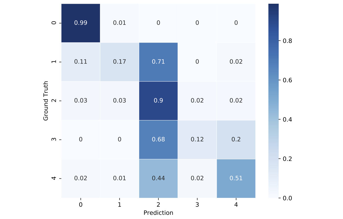
Let's look at the confusion matrix. The matrix illustrates the advantages of the fine-tuned model over the pre-trained CNN and indicates a better performance in classifying mild stages of the DR. However, we also observe that the model classifies too many examples as moderate (class = 2).
#collapse-hide

# construct confusion matrx
oof_preds_round = oof_preds.copy()
cm = confusion_matrix(train['diagnosis'], oof_preds_round)
cm = cm.astype('float') / cm.sum(axis = 1)[:, np.newaxis]
annot = np.around(cm, 2)

# plot matrix
fig, ax = plt.subplots(figsize = (8, 6))
sns.heatmap(cm, cmap = 'Blues', annot = annot, lw = 0.5)
ax.set_xlabel('Prediction')
ax.set_ylabel('Ground Truth')
ax.set_aspect('equal')
Inference
Let's now produce some predictions for the test set!
We aggregate predictions from the models trained during the cross-validation loop. To do so, we extract class scores from the last fully-connected layer and define class predictions as the classes with the maximal score. Next, we average predictions of the 4 networks trained on different combinations of the training folds.
#collapse-hide

##### TRANSFORMATIONS

# parameters
batch_size = 25
image_size = 256

# test transformations
test_trans = transforms.Compose([transforms.ToPILImage(),
                                  transforms.RandomHorizontalFlip(),
                                  transforms.RandomVerticalFlip(),
                                  transforms.ToTensor()])


##### DATA LOADER

# create dataset
test_dataset = EyeTestData(data      = test,
                           directory = '../input/aptos2019-blindness-detection/test_images',
                           transform = test_trans)

# create data loader
test_loader = torch.utils.data.DataLoader(test_dataset,
                                          batch_size  = batch_size,
                                          shuffle     = False,
                                          num_workers = 4)


##### MODEL ARCHITECTURE

# model name
model_name = 'enet_b4'

# initialization function
def init_model(train = True, trn_layers = 2):

    ### training mode
    if train == True:

        # load pre-trained model
        model = EfficientNet.from_pretrained('efficientnet-b4', num_classes = 5)

        # freeze first layers
        for child in list(model.children())[:-trn_layers]:
            for param in child.parameters():
                param.requires_grad = False


    ### inference mode
    if train == False:

        # load pre-trained model
        model = EfficientNet.from_name('efficientnet-b4')
        model._fc = nn.Linear(model._fc.in_features, 5)

        # freeze all layers
        for param in model.parameters():
            param.requires_grad = False


    ### return model
    return model


# check architecture
model = init_model(train = False)
We also use test-time augmentations by creating 4 versions of the test images with random augmentations (horizontal and vertical flips) and average predictions over the image variants. The final prediction is an average of 4 models times 4 image variants.
#collapse-show

# validation settings
num_folds = 4
tta_times = 4

# placeholders
test_preds = np.zeros((len(test), num_folds))
cv_start   = time.time()

# prediction loop
for fold in tqdm(range(num_folds)):

    # load model and sent to GPU
    model = init_model(train = False)
    model.load_state_dict(torch.load('../models/model_{}_fold{}.bin'.format(model_name, fold + 1)))
    model = model.to(device)
    model.eval()

    # placeholder
    fold_preds = np.zeros((len(test), 1))

    # loop through batches
    for _ in range(tta_times):
        for batch_i, data in enumerate(test_loader):
            inputs = data['image']
            inputs = inputs.to(device, dtype = torch.float)
            preds = model(inputs).detach()
            _, class_preds = preds.topk(1)
            fold_preds[batch_i * batch_size:(batch_i + 1) * batch_size, :] += class_preds.cpu().numpy()
    fold_preds = fold_preds / tta_times

    # aggregate predictions
    test_preds[:, fold] = fold_preds.reshape(-1)

# print performance
test_preds_df = pd.DataFrame(test_preds.copy())
print('Finished in {:.2f} minutes'.format((time.time() - cv_start) / 60))
Let's have a look at the distribution of predictions:
#collapse-hide

# show predictions
print('-' * 45)
print('PREDICTIONS')
print('-' * 45)
print(test_preds_df.head())

# show correlation
print('-' * 45)
print('CORRELATION MATRIX')
print('-' * 45)
print(np.round(test_preds_df.corr(), 4))
print('Mean correlation = ' + str(np.round(np.mean(np.mean(test_preds_df.corr())), 4)))

# show stats
print('-' * 45)
print('SUMMARY STATS')
print('-' * 45)
print(test_preds_df.describe())

# show prediction distribution
print('-' * 45)
print('ROUNDED PREDICTIONS')
print('-' * 45)
for f in range(num_folds):
    print(np.round(test_preds_df[f]).astype('int').value_counts(normalize = True))
    print('-' * 45)

# plot densities
test_preds_df.plot.kde()
The model classifies a lot of images as moderate DR. To reduce the number of such examples, we can change thresholds used to round the averaged predictions into classes. We use the following vector of thresholds: [0.5, 1.75, 2.25, 3.5]. The final prediction is set to zero if the average value is below 0.5; set to one if the average value lies in [0.5, 1.75), etc. This reduces the share of images classified as moderate DR.
#collapse-show

# aggregate predictions
test_preds = test_preds_df.mean(axis = 1).values

# set cutoffs
coef = [0.5, 1.75, 2.25, 3.5]

# rounding
for i, pred in enumerate(test_preds):
    if pred < coef[0]:
        test_preds[i] = 0
    elif pred >= coef[0] and pred < coef[1]:
        test_preds[i] = 1
    elif pred >= coef[1] and pred < coef[2]:
        test_preds[i] = 2
    elif pred >= coef[2] and pred < coef[3]:
        test_preds[i] = 3
    else:
        test_preds[i] = 4
We are done! We can now export test_preds as csv and submit it to the competition.
5. Closing words
This blog post provides a complete walkthrough on the project on detecting blindness in the retina images using CNNs. We use image preprocessing to reduce discrepancies across images taken in different clinics, apply transfer learning to leverage knowledge from larger data sets and implement different techniques to improve performance.
If you are still reading this post, you might be wondering about ways to further improve the solution. There are multiple options. First, employing a larger network architecture and increasing the number of training epochs on the pre-training stage has a high potential for a better performance. At the same time, this would require more computing power, which might not be optimal considering the possible use of the automated retina image classification in practice.
Second, image preprocessing can be further improved. During the refinement process, the largest performance gains were attributed to different preprocessing steps. This is a more efficient way to further improve the performance.
Finally, the best solutions of other competitors rely on ensembles of CNNs using different image sizes and/or architectures. Incorporating multiple heterogeneous models and blending their predictions could also improve the proposed solution. Ensembling predictions of models similar to the one discussed in this post is what helped me to place in the top 9% of the leaderboard.
Liked the post? Share it on social media!
You can also buy me a cup of coffee to support my work. Thanks!
